Finding Homogeneous and Particular Solution From Transfer Function
Introduction: System Analysis
Once appropriate mathematical models of a system have been obtained, either in state-space or transfer function form, we may then analyze these models to predict how the system will respond in both the time and frequency domains. To put this in context, control systems are often designed to improve stability, speed of response, steady-state error, or prevent oscillations. In this section, we will show how to determine these dynamic properties from the system models.
Key MATLAB commands used in this tutorial are: tf , ssdata , pole , eig , step , pzmap , bode , linearSystemAnalyzer
Run Live Script Version in MATLAB Online
Contents
- Time Response Overview
- Frequency Response Overview
- Stability
- System Order
- First-Order Systems
- Second-Order Systems
Time Response Overview
The time response represents how the state of a dynamic system changes in time when subjected to a particular input. Since the models we have derived consist of differential equations, some integration must be performed in order to determine the time response of the system. For some simple systems, a closed-form analytical solution may be available. However, for most systems, especially nonlinear systems or those subject to complicated inputs, this integration must be carried out numerically. Fortunately, MATLAB provides many useful resources for calculating time responses for many types of inputs, as we shall see in the following sections.
The time response of a linear dynamic system consists of the sum of the transient response which depends on the initial conditions and the steady-state response which depends on the system input. These correspond to the homogenous (free or zero input) and the particular solutions of the governing differential equations, respectively.
Frequency Response Overview
All the examples presented in this tutorial are modeled by linear constant coefficient differential equations and are thus linear time-invariant (LTI). LTI systems have the extremely important property that if the input to the system is sinusoidal, then the steady-state output will also be sinusoidal at the same frequency, but, in general, with different magnitude and phase. These magnitude and phase differences are a function of the frequency and comprise the frequency response of the system.
The frequency response of a system can be found from its transfer function in the following way: create a vector of frequencies (varying between zero or "DC" to infinity) and compute the value of the plant transfer function at those frequencies. If  is the open-loop transfer function of a system and
  is the frequency vector, we then plot
  versus . Since is a complex number, we can plot both its magnitude and phase (the Bode Plot) or its position in the complex plane (the Nyquist Diagram). Both methods display the same information, but in different ways.
Stability
For our purposes, we will use the Bounded Input Bounded Output (BIBO) definition of stability which states that a system is stable if the output remains bounded for all bounded (finite) inputs. Practically, this means that the system will not "blow up" while in operation.
The transfer function representation is especially useful when analyzing system stability. If all poles of the transfer function (values of  for which the denominator equals zero) have negative real parts, then the system is stable. If any pole has a positive real part, then the system is unstable. If we view the poles on the complex s-plane, then all poles must be in the left-half plane (LHP) to ensure stability. If any pair of poles is on the imaginary axis, then the system is marginally stable and the system will tend to oscillate. A system with purely imaginary poles is not considered BIBO stable. For such a system, there will exist finite inputs that lead to an unbounded response. The poles of an LTI system model can easily be found in MATLAB using the pole command, an example of which is shown below:
s = tf('s'); G = 1/(s^2+2*s+5) pole(G) G = 1 ------------- s^2 + 2 s + 5 Continuous-time transfer function. ans = -1.0000 + 2.0000i -1.0000 - 2.0000i
Thus this system is stable since the real parts of the poles are both negative. The stability of a system may also be found from the state-space representation. In fact, the poles of the transfer function are the eigenvalues of the system matrix  . We can use the eig command to calculate the eigenvalues using either the LTI system model directly, eig(G), or the system matrix as shown below.
[A,B,C,D] = ssdata(G); eig(A)
ans = -1.0000 + 2.0000i -1.0000 - 2.0000i
System Order
The order of a dynamic system is the order of the highest derivative of its governing differential equation. Equivalently, it is the highest power of in the denominator of its transfer function. The important properties of first-, second-, and higher-order systems will be reviewed in this section.
First-Order Systems
First-order systems are the simplest dynamic systems to analyze. Some common examples include mass-damper systems and RC circuits.
The general form of the first-order differential equation is as follows
(1) 
The form of a first-order transfer function is
(2) 
where the parameters  and
and  completely define the character of the first-order system.
DC Gain
The DC gain, , is the ratio of the magnitude of the steady-state step response to the magnitude of the step input. For stable transfer functions, the Final Value Theorem demonstrates that the DC gain is the value of the transfer function evaluated at = 0. For first-order systems of the forms shown, the DC gain is  .
.
Time Constant
The time constant of a first-order system is  which is equal to the time it takes for the system's response to reach 63% of its steady-state value for a step input (from zero initial conditions) or to decrease to 37% of the initial value for a system's free response. More generally, it represents the time scale for which the dynamics of the system are significant.
Poles/Zeros
First-order systems have a single real pole, in this case at  . Therefore, the system is stable if
  is positive and unstable if is negative. Standard first-order system have no zeros.
Step Response
We can calculate the system time response to a step input of magnitude  using the following MATLAB commands:
k_dc = 5; Tc = 10; u = 2; s = tf('s'); G = k_dc/(Tc*s+1) step(u*G) G = 5 -------- 10 s + 1 Continuous-time transfer function.

Note: MATLAB also provides a powerful graphical user interface for analyzing LTI systems which can be accessed using the syntax linearSystemAnalyzer('step',G).
If you right-click on the step response graph and select Characteristics, you can choose to have several system metrics overlaid on the response: peak response, settling time, rise time, and steady-state.
Settling Time
The settling time,  , is the time required for the system output to fall within a certain percentage (i.e. 2%) of the steady-state value for a step input. The settling times for a first-order system for the most common tolerances are provided in the table below. Note that the tighter the tolerance, the longer the system response takes to settle to within this band, as expected.
| 10% | 5% | 2% | 1% |
| Ts=2.3/a=2.3Tc | Ts=3/a=3Tc | Ts=3.9/a=3.9Tc | Ts=4.6/a=4.6Tc |
Rise Time
The rise time,  , is the time required for the system output to rise from some lower level x% to some higher level y% of the final steady-state value. For first-order systems, the typical range is 10% - 90%.
Bode Plots
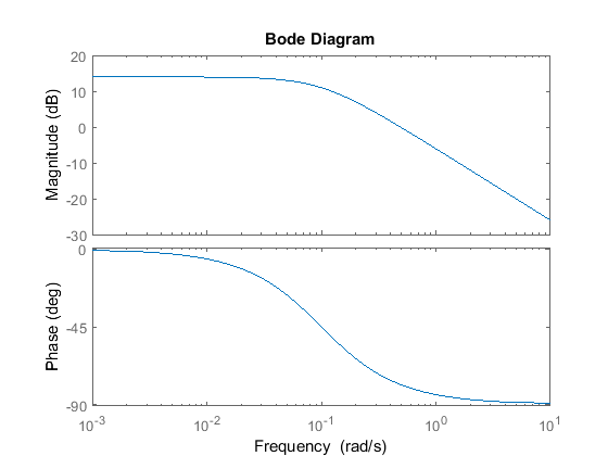
Bode diagrams show the magnitude and phase of a system's frequency response, , plotted with respect to frequency . We can generate the Bode plot of a system  in MATLAB using the syntax bode(G) as shown below.
bode(G)
Again the same results could be obtained using the Linear System Analyzer GUI, linearSystemAnalyzer('bode',G).
Bode plots employ a logarithmic frequency scale so that a larger range of frequencies are visible. Also, the magnitude is represented using the logarithmic decibel unit (dB) defined as:
(3) 
As with the frequency axis, the decibel scale allows us to view a much larger range of magnitudes on a single plot. Also, as we shall see in subsequent tutorials, when components and controllers are placed in series, the transfer function of the overall system is the product of the individual transfer functions. Using the dB scale, the magnitude plot of the overall system is simply the sum of the magnitude plots of the individual transfer functions. The phase plot of the overall system is also just the sum of the individual phase plots.
The low frequency magnitude of the first-order Bode plot is  . The magnitude plot has a bend at the frequency equal to the absolute value of the pole (ie.
  ), and then decreases 20 dB for every factor of ten increase in frequency (slope = -20 dB/decade). The phase plot is asymptotic to 0 degrees at low frequencies, and asymptotic to -90 degrees at high frequencies. Between frequency 0.1a and 10a, the phase changes by approximately -45 degrees for every factor of ten increase in frequency (-45 degrees/decade).
We will see in the Frequency Methods for Controller Design Section how to use Bode plots to calculate closed-loop stability and performance of feedback systems.
Second-Order Systems
Second-order systems are commonly encountered in practice, and are the simplest type of dynamic system to exhibit oscillations. Examples include mass-spring-damper systems and RLC circuits. In fact, many true higher-order systems may be approximated as second-order in order to facilitate analysis.
The canonical form of the second-order differential equation is as follows
(4) 
The canonical second-order transfer function has the following form, in which it has two poles and no zeros.
(5) 
The parameters ,  , and
, and  characterize the behavior of a canonical second-order system.
DC Gain
The DC gain, , again is the ratio of the magnitude of the steady-state step response to the magnitude of the step input, and for stable systems it is the value of the transfer function when  . For the forms given,
(6) 
Damping Ratio
The damping ratio is a dimensionless quantity charaterizing the rate at which an oscillation in the system's response decays due to effects such as viscous friction or electrical resistance. From the above definitions,
(7) 
Natural Frequency
The natural frequency is the frequency (in rad/s) that the system will oscillate at when there is no damping,  .
.
(8) 
Poles/Zeros
The canonical second-order transfer function has two poles at:
(9) 
Underdamped Systems
If  , then the system is underdamped. In this case, both poles are complex-valued with negative real parts; therefore, the system is stable but oscillates while approaching the steady-state value. Specifically, the natural response oscillates with the damped natural frequency,
  (in rad/sec).
k_dc = 1; w_n = 10; zeta = 0.2; s = tf('s'); G1 = k_dc*w_n^2/(s^2 + 2*zeta*w_n*s + w_n^2); pzmap(G1) axis([-3 1 -15 15]) 
step(G1) axis([0 3 0 2])

Settling Time
The settling time, , is the time required for the system ouput to fall within a certain percentage of the steady-state value for a step input. For a canonical second-order, underdamped system, the settling time can be approximated by the following equation:
(10) 
The settling times for the most common tolerances are presented in the following table:
| 10% | 5% | 2% | 1% |
| Ts=2.3/(zeta*w_n) | Ts=3/(zeta*w_n) | Ts=3.9/(zeta*w_n) | Ts=4.6/(zeta*w_n) |
Percent Overshoot
The percent overshoot is the percent by which a system's step response exceeds its final steady-state value. For a second-order underdamped system, the percent overshoot  is directly related to the damping ratio by the following equation. Here, is a decimal number where 1 corresponds to 100% overshoot.
(11) 
For second-order underdamped systems, the 1% settling time, , 10-90% rise time, , and percent overshoot, , are related to the damping ratio and natural frequency as shown below.
(12) 
(13) 
(14) 
Overdamped Systems
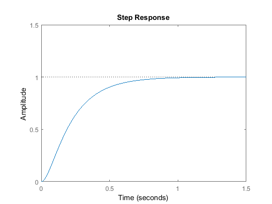
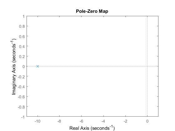
If  , then the system is overdamped. Both poles are real and negative; therefore, the system is stable and does not oscillate. The step response and a pole-zero map of an overdamped system are calculated below:
zeta = 1.2; G2 = k_dc*w_n^2/(s^2 + 2*zeta*w_n*s + w_n^2); pzmap(G2) axis([-20 1 -1 1])

step(G2) axis([0 1.5 0 1.5])
Critically-Damped Systems
If  , then the system is critically damped. Both poles are real and have the same magnitude,
  . For a canonical second-order system, the quickest settling time is achieved when the system is critically damped. Now change the value of the damping ratio to 1, and re-plot the step response and pole-zero map.
zeta = 1; G3 = k_dc*w_n^2/(s^2 + 2*zeta*w_n*s + w_n^2); pzmap(G3) axis([-11 1 -1 1])
step(G3) axis([0 1.5 0 1.5])

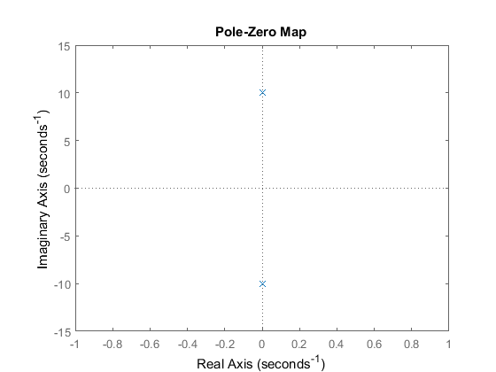
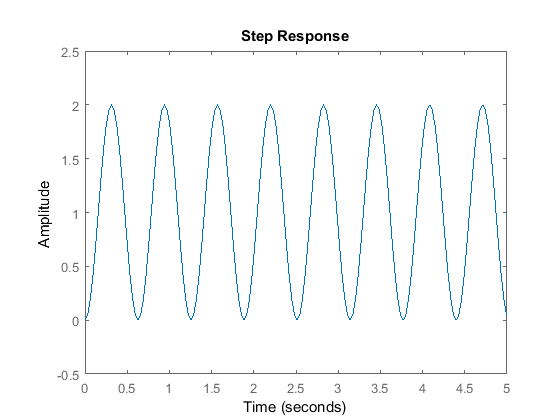
Undamped Systems
If , then the system is undamped. In this case, the poles are purely imaginary; therefore, the system is marginally stable and the step response oscillates indefinitely.
zeta = 0; G4 = k_dc*w_n^2/(s^2 + 2*zeta*w_n*s + w_n^2); pzmap(G4) axis([-1 1 -15 15])
step(G4) axis([0 5 -0.5 2.5])
Bode Plot
We show the Bode magnitude and phase plots for all damping conditions of a second-order system below:
bode(G1,G2,G3,G4) legend('underdamped: zeta < 1','overdamped: zeta > 1','critically-damped: zeta = 1','undamped: zeta = 0')

The magnitude of the bode plot of a second-order system drops off at -40 dB per decade in the limit, while the relative phase changes from 0 to -180 degrees. For underdamped systems, we also see a resonant peak near the natural frequency, = 10 rad/s. The size and sharpness of the peak depends on the damping in the system, and is charaterized by the quality factor, or Q-Factor, defined below. The Q-factor is an important property in signal processing.
(15) 

All contents licensed under a Creative Commons Attribution-ShareAlike 4.0 International License.
Finding Homogeneous and Particular Solution From Transfer Function
Source: https://ctms.engin.umich.edu/CTMS/index.php?example=Introduction§ion=SystemAnalysis